GLIMS algorithm document |
(under development, draft version)
Definitions & Abbreviations
Pre-processing and image corrections
- Georeferencing
- Orthorectification
- Atmospheric corrections
- ...
Glacier mapping
- Boundaries considered
- Multispectral classification
- Multidimensional classification
- Glacier basin creation
- ...
Ice velocity measurements
- Correlation of repeated optical imagery
- ...
DEM generation
- DEM-generation from ASTER
- ...
Change detection
- Ice / snow / water
- ...
Literature
Authors
Contact, Links & Publications
Definitions & Abbreviations |
- Reflectance L = offset + gain * DN
- at satellite planetary reflectance R = (L * pi * d^2) / (S * cos(theta))
- atmosphere and illumination corrected (requires DEM): A
.
- DN: digital number
- DOS: dark object subtraction
- FCC: false colour composite
- IHS: Intensity - Hue - Saturation
- ISODATA: iterative self organizing data analysis
- MIR: middle infrared
- SGI2000: Swiss Glacier Inventory 2000
- SWIR: shortwave infrared
- TIR: thermal infrared
- VIS: visible
- VNIR: visible and near infrared
- .
| UP | HOME | ||||
Glacier mapping |
Manual |
|
Name: |
Manual glacier delineation |
Description: |
Cursor tracking of glacier boundaries on contrast enhanced FCCs, either pixel by pixel (raster-based) or with the image as a background using GIS (vector-based). |
Pros: |
Highest accuracy, inclusion of debris-covered ice, exclusion of adjacent snow-fields, works also for panchromatic images (e.g. from SPOT, IRS-1C, Ikonos). |
Cons: |
Laborious (time) for a large number of glaciers, not consistent through image, requires interpretation from specialist, difficult interpretation of pan images. |
Notes: |
Required time increases with decreasing sensor resolution. Often the only method for delineation of debris-covered glacier ice. |
Sensors: |
Works with all optical sensors (possibly also SAR) |
Literature: |
Rott & Markl 1989, Hall et al. 1992, Williams & Hall 1993, Williams et al. 1997 |
Application within SGI2000: |
Glacier outlines on Ikonos pan and IHS-fused TM / SPOT pan and TM / IRS-1C pan imagery. Debris-cover delineation on TM543 composites (with classified glacier-map as an overlay). |
Ratio |
|
Name: |
Ratio images |
Description: |
Division of two spectral bands and thresholding to obtain black and white map |
Pros: |
Fast, simple and robust |
Cons: |
Vegetation in shadow and turbid lakes are partly classified as glaciers |
Notes: |
|
Sensors: |
TM: TM4 / TM5 with DNs reveals best results. For deep shadows TM3 / TM5 is better.
ASTER: ASTER VNIR resolution 15m, SWIR 30m. ASTER 2 = TM 3, ASTER 3 = TM 4, ASTER 4 = TM 5. ASTER 3 / ASTER 4 tested. Either band 3 or 4 have to be resampled. Results similar to TM. |
Literature: |
Della Ventura et al. 1987, Hall et al. 1988, Bayr et al. 1994, Rott 1994, Jacobs et al. 1997, Paul 2001, Paul 2002, Paul in prep |
Application within SGI2000: |
TM3 / TM5 and TM4 / TM5 with DNs, L, R and A |
Example: |
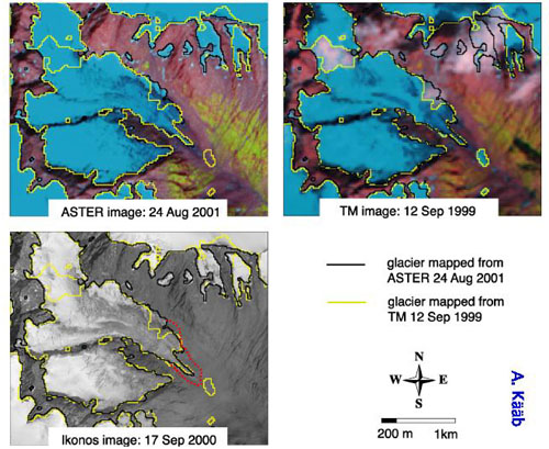
Glacier outlines in the Chelenalp valley, Swiss Alps, as mapped automatically from an ASTER image of 24 Aug 2001 and a Landsat TM image of 12 Sep 1999. The debris-covered tongue of Chelenalpgletscher is manually delineated from an Ikonos image of 17 Sep 2000 (red dashed line). Upper left image: RGB-composite of ASTER 4 3 2, 15m resolution. Upper right image: RGB-composite of TM 5 4 3, 30m resolution. Lower left image: Ikonos pan band, 1m resolution. Glacier outlines as automatically computed from a TM 4/5 ratio are shown in yellow and those from an ASTER 3/4 ratio in black. Largest differences between the TM and the ASTER glacier mapping are due to snow remains in 2001 and clouds in 1999. Largest differences of the TM and ASTER glacier mapping compared to the Ikonos image occur for debris-covered ice which is not detected from the multi-spectral ratios. (from Kääb et al. in press). |
NDSI |
|
Name: |
Normalized Difference Snow Index (NDSI) |
Description: |
Based on differences in spectral properties of snow in VIS and MIR: e.g. (TM2 - TM5) / (TM2 + TM5). Threshold must be carefully selected |
Pros: |
Classification of partly debris-covered pixels (along the glacier perimeter) is somewhat better than with e.g. TM4 / TM5 |
Cons: |
In sunlight, also partly snow-covered pixels are mapped (resulting in too large glacier areas). Accuracy of snow / ice mapping in cast shadow depends on DOS for TM2 (areas too large without correction). |
Notes: |
Usage of L instead of DN doesn't improve classification. Snow / ice separation with higher threshold not possible due to illumination bias in steep topography and shadow |
Sensors: |
|
Literature: |
|
Application within SGI2000: |
NDSI using DN without DOS |
Unsupervised |
|
Name: |
Unsupervised classification |
Description: |
ISODATA clustering is an automatic iterative method which is working on various input bands (somewhat similar to rgb-composites but with more than three channels). Number of clusters (min. & max.) and iterations (max.) required |
Pros: |
Fast, comparable accurate for clean ice in sunlight |
Cons: |
Black box with `trial and error' results, careful interpretation of final classes required, difficulties with glacier ice in shadow |
Notes: |
Not recommended for operational applications |
Sensors: |
|
Literature: |
Aniya et al. 1996, Paul 2001 |
Application within SGI2000: |
Test with 20 and 31 classes and TM bands 1-5 (DN) as input. |
Supervised |
|
Name: |
Supervised classification |
Description: |
Selection and marking of training areas according to specified object classes and final classification with available classifier (e.g. nearest neighbour, parallel epiped, Maximum-Likelihood) |
Pros: |
Comparable accurate for clean ice in sunlight. Integration of pre-processed bands is possible |
Cons: |
Spectral signatures of object classes are scene dependent, reflectance must be calculated otherwise. Selection of appropriate training areas is not straight forward in complex terrain with steep topography (shadows). Classifier works as a black-box. |
Notes: |
May work better in more uniform terrain (spectrally, topography). Worth a try then. |
Sensors: |
|
Literature: |
Gratton et al. 1990, Binaghi et al. 1993, Sidjak & Wheate 1999, Bronge & Bronge 1999, Paul 2001, Paul 2002 |
Application within SGI2000: |
Maximum-Likelihood classification with 10 classes and TM bands 1-5 (EN) as input |
.
= classification using not only spectral data but also DEMs, spectral derivatives, multitemporal data etc.
Debris (F. Paul) |
|
Name: |
Mapping of debris-covered glacier ice |
Description: |
Combined approach, using glacier map from TM4 / TM5, vegetation map from hue component of TM 3, 4 and 5 and slope from DEM. In a first step debris-covered glaciers are assigned to all ice-free and vegetation-free terrain with slope angles less than 23°. In a second step all debris not connected to glacier ice is eliminated. At last manual corrections for debris connected to snow fields or located in flat glacier fore fields is applied. |
Pros: |
Works automatically (steps 1 and 2) and is quite accurate (depending on DEM quality!) |
Cons: |
Manual corrections can be quite intense. Threshold slope angle should be tested. DEM needed. |
Notes: |
Can be used as a first guess or a guide for manual delineation, if more appropriate |
Sensors: |
|
Literature: |
Paul in prep., Paul et al. (2004). |
Application within SGI2000: |
Used in combination with manual debris-cover delineation on a TM543 FCC |
Glacier boundaries delineation from a DEM (B. Raup) |
|
Name: |
Finding glacier boundaries from topography |
Description: |
In the first version, a person clicks an approximate centerline down the glacier. The algorithm then searches out from there to find V-shaped grooves on either side that are concave-up, and which are trough-shaped roughly parallel to the input centerline (i.e. not bowl-shaped). A similar search is done forward from the downhill end of the input centerline. The resulting outline is then filtered in a manner similar to a median filter, but extended to two dimensions. This method could be extended to use seed areas found by multispectral methods, similar to the approach by F. Paul above, obviating the need for analyst-input at the beginning. |
Pros: |
Can find approximate boundaries even for heavily debris-covered glaciers. |
Cons: |
DEM that resolves the edge of the glaciers is needed. The resulting outlines need manual corrections. |
Notes: |
Can be used as a first guess or a guide for manual delineation. |
Sensors: |
DEM from ASTER or better. Tested with AVIRIS-simulated ASTER and USGS DEM.
|
Literature: |
Bruce Raup (NSIDC), a figure (3 D) illustrating this method is in Kieffer (2000) |
Example: |
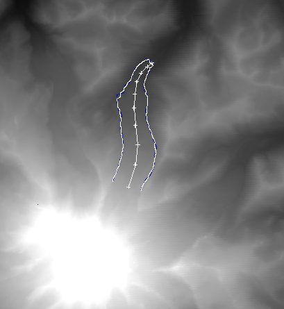
A centerline was clicked down the Winthrop Glacier on Mt. Rainier, Washington, USA. The algorithm determined the boundary, shown in |
Identify ice devides from DEM (W. Manley) |
|
Name: |
Isolate glaciers |
Description: |
Breakes polygones delineating large ice masses into separate "glaciers", based on ice devides. Input: ice polygones (or an ice grid) and coregistered DEM. Procedure: 1. filling of DEM sinks 2. creating flow direction grid 3. finding glacier toes 4. producing watersheds (basins) 5. respective separation of ice polygones into glacier polygons. |
Pros: |
Objective means of differenciating and defining "glaciers" based on the median elevation of ice masses and watershed boundaries |
Cons: |
DEM needed |
Notes: |
Sensitivity to DEM accuracy and resolution not tested. The largely automated process runs in ArcInfo. |
Sensors: |
|
Literature: |
Bill Manley (INSTAAR, Univ. of Colorado) |
| UP | HOME | ||||
Ice velocity measurements |
IMCORR |
|
Name: |
IMCORR |
Description: |
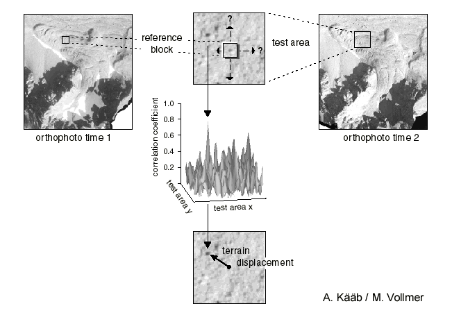
IMCORR takes two images and a series of input parameters and attempts to match small subscenes (called 'chips') from the two images. The program uses a fast fourier transform - based version of a normalized cross-covariance method (see Berenstein, 1983). The most common use of this type of algorithm in image processing is to accurately locate tie-point pairs in two images to coregister them. However, if the images are already coregistered by other means, the algorithm may be used to find the displacements of moving features, provided that the features show little change in their appearance, and that the motion is strictly translational. IMCORR takes as input the image names and sizes, parameters determining search chip size, reference chip size, grid spacing, and output filename. Further, preset offsets of search chip centers may be specified, and subareas of the full image files may be used to restrict the area over which IMCORR attempts to find displacements. At each of the gridpoints IMCORR calculates a correlation index for every location at which the reference chip will entirely fit within the search chip. IMCORR takes the correlation values in the vicinity of the best integer-pixel match and interpolates a peak correlation location to sub-pixel precision. The program returns a file containing the locations of the grid centers for the reference chips, the displacements required to best match the chip pairs (or indicates that none could be found), and several quality control parameters that may be used to evaluate the validity of the match. We use this program to measure glaicer velocities; however, the same program may be useful for other applications. The correlation, peak finding, and error estimation routines in IMCORR are derived from FORTAN subroutines from the Land Analysis System software (LAS) written at NASA Goddard Space Flight Center and USGS Eros Data Center. IMCORR consists of a C code wrapper which makes the use of the routines more straightforward and automated for velocity-mapping applications. |
Pros: |
cf. CIAS |
Cons: |
cf. CIAS |
Notes: |
Free download. Fortran / C |
Sensors: |
All imagery. Well tested among others for Landsat TM.
|
Literature: |
Scambos et al. 1992 |
Link: |
http://nsidc.org/data/velmap/imcorr.html |
CIAS |
|
Name: |
Correlation Image Analyser (Department of Geography, Zurich) |
Description: |
Image pyramid matching using double cross-correlation in feature space.
|
Pros: |
Accurate velocity fields for debris-free and debris-covered glaciers etc. Accuracy of approx. 0.5-1 pixel is mainly dominated by the terrain features, not by the algorithm. In general optical correlation methods are robust and easy to use. |
Cons: |
Image correlation, in general, works not for (1) too slow movements (smaller than the methods significance level), (2) little optical image contrast (e.g. snow etc.), and (3) strong terrain destructions (e.g. shearing, strong melt). |
Notes: |
Written in IDL, i.e. requires IDL run-time licence. If you want to have ice-flow measured from your repeated imagery, feel free to contact Andreas Kääb . |
Sensors: |
All imagery. Tested for aerial imagery (0.1-1 m resolution), Landsat ETM+ pan (15m resolution), ASTER VNIR (15m resolution). Image resolution is THE crucial parameter for image correlation. The better the resolution the better the results.
|
Literature: |
Kääb and Vollmer 2001, Kääb (2002), Kääb et al. (2003) |
Examples: |
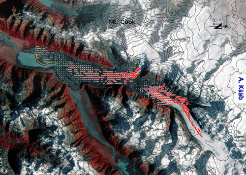
Ice flow vectors for Tasman Glacier, New Zealand, superimposed on an ASTER image of 29 April 2000. Contour lines of 200m interval are computed from the according ASTER DEM. The ice-flow vectors have been derived from automatic image correlation between ASTER images of 29 April 2000 and 7 April 2001. Ice speeds reach 250 m a-1. The striking decrease of ice flow for Tasman Glacier (flowing from the right) at the confluence with Hochstetter Glacier (flowing from the top) indicates a complex interaction between both glaciers. |
Link: |
CIAS |
| UP | HOME | ||||
DEM-generation |
under construction
ASTER DEMs using PCI Orthoengine (Kääb 2002 in press, Kääb et al. in press). Examples.
ASTER DEMs by MacKinnon / Kääb (under development)
ASTER DEMs using LH Systems SOCET SET (to be tested)
...
Authors |
- Alphabetical order
- ...
- Andreas Kääb
- Bill Manley
- Frank Paul
- Bruce Raup
- ...
| UP | HOME | ||||
References |
Ice sheets not considered!
Aniya, M., Sato, H., Naruse, R., Skvarca, P. and Casassa, G. (1996): The use of satellite and airborne imagery to inventory outlet glaciers of the Southern Patagonia Icefield, South America, Photogrammetric Engineering and Remote Sensing, 62, 1361 - 1369.
Bayr, K. J., Hall, D. K. and Kovalick, W. M. (1994): Observations on glaciers in the eastern Austrian Alps using satellite data, International Journal of Remote Sensing, 15, 1733 - 1742.
Binaghi, E. Madella, A., Madella, P. and Rampini, A. (1993): Integration of remote sensing images in a G. I. S. for the study of alpine glaciers, in Winkler (ed.): Remore sensing for monitoring the changing environment of Europe, Balkema, Rotterdam, 173 - 178.
Binaghi, E., Madella, P., Montesano, M. P. and Rampini, A. (1997): Fuzzy contextual classification of multisource remote sensing images, IEEE Transactions on Geoscience and Remote Sensing, GE - 35 (2), 326 - 339.
Bronge, L. B. and Bronge, C. (1999): Ice and snow-type classification in the Vestfold Hills, East Antarctica, using Landsat-TM data and ground radiometer measurements, International Journal of Remote Sensing, 20, 225 - 240.
Della Ventura, A., Rampini, A., Rabagliati,R. and Serandrei Barbero, R. (1983): Glacier monitoring by satellite, Il Nuovo Cimento, C-1, 6, 211 - 221.
Della Ventura, A., Rampini, A. and Serandrei Barbero, R. (1987): Development of a satellite remote sensing technique for the study of alpine glaciers, International Journal of Remote Sensing, 8, 203 - 215.
Dozier, J. (1984): Snow reflectance from Landsat 4 Thematic Mapper, IEEE Transactions on Geoscience and Remote Sensing, GE - 22, 323 - 328.
Dozier, J. (1989): Spectral signature of alpine snow cover from Landsat 5 TM, Remote Sensing of Environment, 28, 9 - 22.
Dozier, J. and Marks, D. (1987): Snow mapping and classification from Landsat Thematic Mapper data, Annals of Glaciology, 9, 97 - 103.
Dowdeswell, J. A. and Cooper, A. P. R. (1986): Digital mapping in polar regions from Landsat photographic products: a case study, Annals of Glaciology, 8, 47 - 50.
Gratton, D. J., Howarth, P. J. and Marceau, D. J. (1990): Combining DEM parameters with Landsat MSS and TM imagery in a GIS for mountain glacier characterization, IEEE Transactions on Geoscience and Remote Sensing, GE - 28, 766 - 769.
Gratton, D. J., Howarth, P. J. and Marceau, D. J. (1993): Using Landsat-5 Thematic Mapper and digital elevation data to determine the net radiation field of a mountain glacier, Remote Sensing of Environment, 43, 315 - 331.
Hall, D. K. and Martinec, J. (1985): Remote sensing of ice and snow, Chapman & Hall.
Hall, D. K., Ormsby, J. P., Bindschadler, R. A. and Siddalingaiah, H. (1987): Characterization of snow and ice zones on glaciers using Landsat Thematic Mapper data, Annals of Glaciology, 9, 104 - 108.
Hall, D. K., Chang, A. T. C. and Siddalingaiah, H. (1988): Reflectances of glaciers as calculated using Landsat 5 Thematic Mapper data, Remote Sensing of Environment, 25, 311 - 321.
Hall, D. K., Bayr, K. J. and Kovalick, W. M. (1989a): Determination of glacier mass balance change using Thematic Mapper data, Proceedings of Eastern Snow Conference, Lake Placid, New York, 7. - 9.6.1988, 192 - 196.
Hall, D. K., Chang, A. T. C., Foster, J. L., Benson, C. S. and Kovalick, W. M. (1989b): Comparison of in situ and Landsat derived reflectances of Alaskan glaciers, Remote Sensing of Environment, 28, 493 - 504.
Hall, D. K., Bindschadler, R. A., Foster, J. L., Chang, A. T. C. and Siddalingaiah, H. (1990): Comparison of in situ and satellite derived reflectances of Forbindels Glacier, Greenland, International Journal of Remote Sensing, 11, 493 - 504.
Hall, D. K., Williams, R. S. Jr. and Bayr, K. J. (1992): Glacier recession in Iceland and Austria, EOS, Transactions of the American Geophysical Union, 73, 129, 135 and 141.
Hall, D. K., Williams, R. S. Jr. and Sigurdsson, O. (1995a): Glaciological Observations on Bruarjökull, Iceland, using synthetic aperture radar and Thematic Mapper satellite data, Annals of Glaciology, 21, 271 - 276.
Hall, D. K., Benson, C. S. and Field, W.O. (1995): Changes of glaciers in Glacier Bay, Alaska, using ground and satellite measurements, Physical Geography, 16, 27 - 41.
Howarth, P. and Ommanney, C. S. (1986): The use of Landsat digital data for glacier inventories, Annals of Glaciology, 8, 90 - 92.
Jacobs, J. D., Simms, E. L. and Simms, A. (1997): Recession of the southern part of Barnes Ice Cap, Baffin Island, Canada, between 1961 and 1993, determined from digital mapping of Landsat TM, Journal of Glaciology, 43, 98 - 102.
Jacobsen, A., Carstensen, A. R. and Kamper, J. (1993): Mapping of satellite derived surface albedo on the Midtluagkat Glacier, Eastern Greenland, using a digital elevation modell and SPOT HRV data, Geografisk Tidsskrift, 93, 6 - 18.
Kääb A., C. Huggel, F. Paul, R. Wessels, B. Raup, H. Kieffer and J. Kargel (2003): Glacier Monitoring from ASTER Imagery: Accuracy and Applications. Proceedings of EARSeL-LISSIG-Workshop Observing our Cryosphere from Space, Bern, March 11 – 13, 2002. EARSeL e Proceedings. 2. 43-53.
Kieffer, H. and others (2000): New Eyes in the Sky Measure Glaciers and Ice Sheets. Eos Transactions, American Geophysical Union, 81 (24), June 13.
Klein A.G. and Isacks, B. L. (1999): Spectral mixture analysis of Landsat Thematic Mapper images applied to the detection of the transient snowline on tropical Andean glaciers. Global and Planetary Change, 22, 139-154.
Knap, W.H. (1998): Satellite-derived and ground-based measurements of the surface albedo of glaciers, PhD Dissertation, University of Utrecht, 173 p.
Koelemeijer, R., Oerlemanns, J. and Tjemkes, S. (1993): Surface reflectance of Hintereisferner, Austria, from Landsat 5 TM imagery, Annals of Glaciology, 17, 17 - 22.
Krimmel, R. M. and Meier, M.F. (1975): Glacier applications of ERTS - 1 images, Journal of Glaciology, 15, 391 - 402.
Li, Z., Sun, W. and Zeng, Q. (1998): Measurements of glacier variation in the Tibetan Plateau using Landsat data, Remote Sensing of Environment, 63, 258 - 264.
Lodwick, G. D. and Paine, S. H. (1985): A digital elevation model of the Barnes Ice-cap derived from Landsat MSS data, Photogrammetric Engineering and Remote Sensing, 51, 1937 - 1944.
Marshall, G. J., Rees, W. G. and Dowdeswell, J. A. (1995): The discrimination of glacier facies using multitemporal ERS - 1 SAR data, in: Askne, J. (ed.), Sensors and environmental applications of remote sensing, Balkema, Rotterdam, 263 -269.
Østrem, G. (1975): ERTS - 1 data in glaciology - an effort to monitor glacier mass balance from satellite imagery, Journal of Glaciology, 15, 403 - 415.
Orheim, O. and Lucchitta, B.K. (1987): Snow and ice studies by Thematic Mapper and Multispectral Scanner Landsat images, Annals of Glaciology, 9, 109 - 118.
Paul F., C. Huggel and A. Kääb (2004): Combining satellite multispectral image data and a digital elevation model for mapping debris-covered glaciers Remote Sensing of Environment. 89(4). 510-518.
Rott, H. (1976): Analyse der Schneeflächen auf Gletschern der Tiroler Zentralalpen aus Landsat Bildern, Zeitschrift für Gletscherkunde und Glazialgeologie, 12, 1 - 28.
Rott, H. (1994): Thematic studies in alpine areas by means of polarimetric SAR and optical imagery, Advances in Space Research, 14, 217 - 226.
Rott, H. and Markl, G. (1989): Improved snow and glacier monitoring by the Landsat Thematic Mapper, Proceedings of a workshop on Landsat Themaic Mapper applications, ESA, SP - 1102, 3 - 12.
Rundquist, D. C., Collins, S. C., Barnes, R. B., Bussom, D. E., Samson, S. A. and Peake, J.S. (1980): The use of Landsat digital information for assessing glacier inventory parameters, IAHS, 126, 321 - 331.
Serandrei-Barbero, R., Rabagliati, R., Binaghi, E. & Rampini, A. (1999): Glacial retreat in the 1980s in the Breonie, Aurine and Pusteresi groups (eastern Alps, Italy) in Landsat TM images, Hydrological Sciences Journal, 44 (2), 279-296.
Sidjak, R. W. and Wheate, R. D. (1999): Glacier mapping of the Illecillewaet icefield, British Columbia, Canada, using, Landsat TM and digital elevation data, International Journal of Remote Sensing, 20, 273 - 284.
Warren, S. G. (1982): Optical properties of snow, Reviews of Geophysics and Space Physics., 20, 67 - 89.
Williams, R.S., Jr. (1983): Remote sensing of glaciers, in: Geological Applications (Williams, R. S., Jr., author-editor), Manual of Remote Sensing, 2nd ed. (Colwell, R. N., ed.-in chief), V. II, Interpretation and Applications (Estes, J. E. and Thorley, G. A., eds.) Falls Church, VA, American Society of Photogrammetry, 1852 - 1866.
Williams, R.S., Jr. (1987): Satellite remote sensing of Vatnajökull, Iceland, Annals of Glaciology, 9, 119 - 125.
Williams, R. S., Jr. and Ferrigno, J. G. (1988): Satellite image atlas of glaciers of the world - Europe, U.S. Geol. Survey, Prof. Paper, 1386 - E, 164 pages.
Williams, R. S., Jr., Hall, D. K. and Benson, C. S. (1991): Analysis of glacier facies using satellite techniques, Journal of Glaciology, 37, 120 - 127.
Williams, R. S., Jr. and Hall, D. K. (1993): Glaciers, in: Gurey, R. J., Foster, J. L. and Parkinson, C. L., Atlas of satellite observations related to global change, Cambridge University Press, 401 - 421.
Williams, R. S., Jr., Hall, D. K., Sigurdsson, O. and Chien, J. Y. L (1997): Comparisson of satellite-derived with ground-based measurements of the fluctuations of the margins of Vatnajökull, Iceland, 1973-1992, Annals of Glaciology, 24, 72 -80.
Williams, R. S.,Jr. and Hall, D. K. (1998): Use of remote-sensing techniques, in: Haeberli, W., Hoelzle, M., and Suter, S., Into the second century of worldwide glacier monitoring: prospects and strategies, UNESCO Publishing, 97 - 111.
Winther, J. G. (1993): Landsat TM derived and in situ summer reflectance of glaciers in Svalbard, Polar Reserach, 12, 37 - 55.
Zeng, Q., Cao, M., Feng, X., Liang, F., Chen, X. and Sheng, W. (1983): A study of spectral reflection characteristics for snow, ice and water in the north of China, IAHS, 145, 451-462.
| UP | HOME | ||||
Contact, Links & Publications |
For any comments or questions please contact Andreas Kääb.
Selected links on remote sensing algorithms for glacier analysis:
Swiss Glacier Inventory 2000 / Frank Paul
...
Selected GLIMS publication downloads on comparisons of remote sensing algorithms for glacier analysis:
Paul, F. (2001): Evaluation of different methods for glacier mapping using Landsat TM. EARSeL Workshop on Remote Sensing of Land Ice and Snow, Dresden, 16.-17.6.2000. EARSeL eProceedings, 1, 239-245, CD-ROM. [PDF 0.5 MB]
Paul F., A. Kääb, M. Maisch, T. Kellenberger and W. Haeberli (2002): The new remote-sensing-derived Swiss glacier inventory: I. Methods. Annals of Glaciology. 34. 355-361.
Kääb A., C. Huggel, F. Paul, R. Wessels, B. Raup, H. Kieffer and J. Kargel (2003): Glacier Monitoring from ASTER Imagery: Accuracy and Applications. EARSeL Proceedings. LIS-SIG Workshop. Berne, March 11-13, 2002.
Kääb A (2002): Monitoring high-mountain terrain deformation from repeated air- and spaceborne optical data: examples using digital aerial imagery and ASTER data. ISPRS Journal of Photogrammetry & Remote Sensing. 57 (1-2). 39-52.
| UP | HOME | ||||
May 2004 - A. Kääb